Pools and memory
Imagine we have a pool (of infected people, scared people, whatever). We have an incidence rate \(i(t)\) that explains how things enter. We describe how they stay either in terms of a kernel \(k(\tau)\) (if you enter at time \(t\), this is the probability of still being there at time \(t+\tau\), or a hazard \(h(\tau) = -k'(\tau)/k(\tau)\), where the prime represents the simple derivative. \(h\) represents the instantaneous probability rate of leaving, given that you are still present.
We will only talk about hazard if \(k\) is non-decreasing (representing people “entering” at rate \(i\) and then leaving. This is a straightforward assumption if we are counting, say, infected people, but not for mework for more complicated structures like an exposed and an infectious class, or delayed-onset fear.
Change through time
The number in the pool at time \(t\) is:
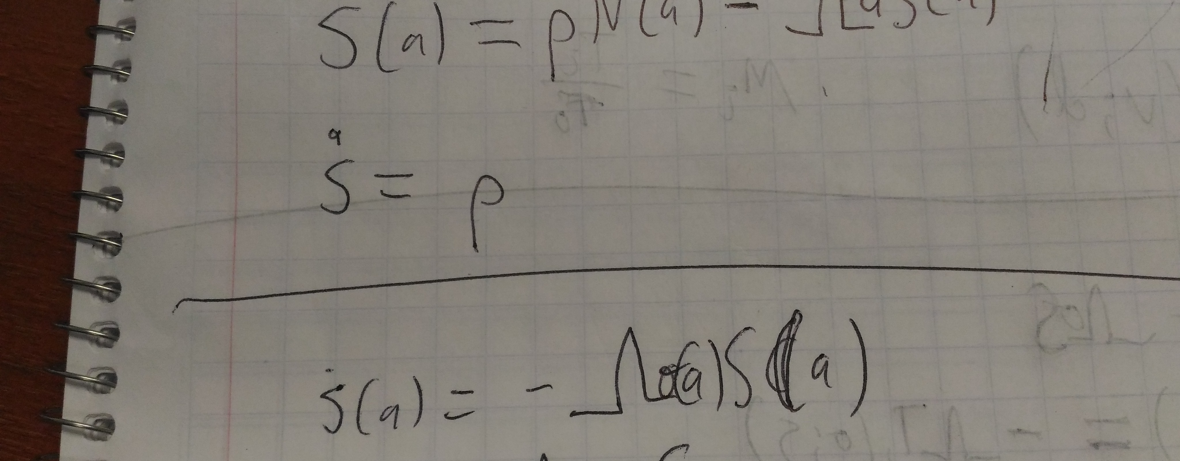
\[\phi(t) = \int_0^\infty i(t-\tau) k(\tau) d\tau\]The time derivative is
\[\dot\phi(t) = \int_0^\infty i'(t-\tau) k(\tau) d\tau,\]which simplifies to
\[\dot\phi(t) = k(0) i(t) + \int_0^\infty k'(\tau) i(t-\tau) d\tau.\]This doesn’t look simpler, but is, because \(i(t)\) is a general function, provided from outside, whereas \(k(\tau)\) is something that we specify. The cool way to do this simplification is by integrating by parts; the easy is by reparameterizing the integral using \(s=t-\tau\).
Constant hazard
Under the hazard assumption, we have:
\[\dot\phi(t) = k_0 i(t) - \int_0^\infty h(\tau) k(\tau) i(t-\tau) d\tau.\]If we assume hazard is constant (\(h(\tau)\equiv h\)), we can pull \(h\) out of the integral, and recover the original definition of \(\phi\) on the RHS:
\[\dot\phi(t) = k_0 i(t) - h\phi.\]It might be fun to see what other rearrangements can be done with the first integral above …
Scenarios
The natural limiting cases for a fear scenario are:
- Fear proportional to incidence (II): let \(h \to \infty\)
- Fear proportional to cumulative incidence (CI): let \(h \to 0\).
- Fear proportional to prevalence (P): let \(k(\tau) \propto \ell(\tau)\), where \(\ell\) is the kernel describing the infection process
Apples and oranges
Is there a natural way to set parameters to compare these scenarios? Not really.
We can compare CI to P using \(k_0=1\), but this will always make the CI look stronger (we are comparing a long memory to a short memory without normalizing)
There is also a natural normalization, which we already used for II. More generally, we set \(k_0\) so that the kernel function integrates to 1. This will generally make shorter memories seem more effective: if we really attempt to take the CI limit with this normalization, we find that CI has zero effect within a finite time window, so that’s definitely not what we want.
This normalization makes good sense for long time periods. In particular, any memory function should give the same equilibrium value of \(\phi\), for systems which reach equilibrium. To do this correctly with CI, you would need \(h\) to be slow compared to the disease process, but fast compared to the whole time scale of dynamics you were studying.
We could also just try different values of \(h\) (or distributions of \(k\)) but admit that we can’t directly compare their effectiveness parameters.
